Polyhedra whose vertex coordinates have no closed form formula
The cube has the nice symmetric set of Cartesian vertex coordinates \( (\pm 1, \pm 1, \pm 1) \). These give it an edge length of \( 2 \), but if you want any other number \( s \) just scale by \( s/2 \). Similarly, the regular octahedron can be give coordinates that are all the possible permutations of \( (0, 0, \pm 1) \), and the regular tetrahedron can be given coordinates that are a subset of the cube's vertices, the ones with an even number of plus signs; in both cases the scale factor involves the square root of two. The regular dodecahedron can be formed from the eight vertices of a cube by adding twelve more vertices with coordinates formed by cyclically permuting \( (0, \pm\varphi, \pm 1/\varphi) \), where \( \varphi \) is the golden ratio; its scaling factor also involves the golden ratio. And the regular icosahedron, with side length \( 2 \) (like the cube, and with the same scaling factor), has coordinates given by all cyclic permutations of \( (0, \pm 1, \pm\varphi) \). The three subsets of four vertices having the same cyclic permutation as each other form three golden rectangles, which interlock in the pattern of the Borromean rings and have the icosahedron as their convex hull:

(image from Wikimedia commons)
It's also possible to make irregular variants of these polyhedra (or of any other polyhedron), with the same combinatorial structure and integer coordinates. For instance, the cyclic permutations of \( (0, \pm 1, \pm 2) \) give an irregular icosahedron. Finding small integer coordinates for a polyhedron combinatorially equivalent to the regular dodecahedron makes an amusing exercise, and bounding how big the coordinates need to be to realize all polyhedra remains an intriguing open problem.
Given all this, you might be forgiven for thinking that every polyhedron has a nice closed-form formula for its vertex coordinates. But when the geometry and not just the combinatorics of the polyhedron is specified, it's not true, even when the polyhedron's faces are particularly simple (say, integer-sided triangles).
To begin with, what is the input? One reasonable choice for how to describe a polyhedron is to give a net, a set of planar polygons (the faces of the polyhedron) connected to each other edge-to-edge, with instructions for how to glue the remaining edges together. It's a useful way of making polyhedral models out of paper, but a bit problematic from the point of view of theoretical algorithms, because we still don't know whether all polyhedra have nets. A bit more abstractly, we could specify the shape of each face, and the gluing pattern of the edges, without requiring that the faces form a connected net in the plane. By Cauchy's theorem, this is enough to determine the whole geometry. But it still has the issue that the shapes won't always glue together the way you think they should. Instead, a standard alternative description of the input to the problem is to describe its development: the metric space you get from shortest paths that stay within its surface. This can again be done by gluing together polygons. As long as the resulting complex has the topology of a sphere and each vertex has a total angle strictly less than \( 2 \pi \), it will form a unique convex polyhedron by Alexandrov's uniqueness theorem, but not necessarily one with the input polygons as its faces. The examples that I'll use to show that closed-form formulas don't exist can be given in any of these three forms (nets, gluing patterns of faces, or developments), and their faces have particularly simple shapes: isosceles triangles with integer edge lengths.
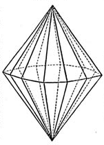
A first hint that a closed-form formula might not exist comes from a paper by Maksym Fedorchuk and Igor Pak, "Rigidity and polynomial invariants of convex polytopes", Duke Math. J. 2005. They use regular bipyramids (the convex hulls of a convex polygon within a plane, a point above the polygon, and a point below the polygon, but with variable edge lengths) to show that the polynomials describing the coordinates as a function of edge lengths can have exponentially high degree. But of course high degree doesn't necessarily imply no closed form solution: regardless of how high \( d \) is, the polynomial \( x^d - 2 \) has a root with the simple closed form solution \( 2^{1/d} \).
(image from Wikimedia commons)
In part because of this result, a later paper by Kane, Price, and Demaine ("A pseudopolynomial algorithm for Alexandrov's theorem", WADS 2009) gave up on trying to find an exact algebraic solution for the vertex coordinates, and instead showed that (for developments as input) an accurate numerical approximation to a polyhedral realization could be found in pseudopolynomial time, using methods involving the solution to differential equations.
So we know that the realization for a given input has an algebraic solution, but we don't know of a good closed form solution, and instead practical algorithms use numerical methods that converge reasonably quickly. Those characteristics should sound familiar: they're the same as the background to my paper "The Galois Complexity of Graph Drawing" (with Bannister, Devanny, and Goodrich, JGAA 2015). In that paper, we showed that many graph drawing problems with similar characteristics could not be solved in algebraic computation tree models of computation augmented with a polynomial-root-finding primitive, in two variations: the primitive could either compute \( d \)th roots of given numbers, for arbitrarily large \( d \), or it could compute roots of more complicated polynomials but only of bounded degree. In both cases, we showed that this computational model is incapable of representing the exact solution to the graph drawing problems we studied, regardless of how much time it spends in searching for the solution.
In the blog post in which I announced the preprint version of the Galois complexity paper, I described similar results for an even simpler geometric problem: given a cycle graph with specified edge lengths, draw it in the plane so that all the vertices are in cycle order around a circle. The special case of this problem with all edge lengths equal to each other and the cycle length derived from a Sophie Germain prime cannot be drawn by a computation tree using bounded-degree-polynomial-root primitives, and an example found by Varfolomeev (2004) shows that it cannot be drawn by a computation tree using arbitrary-degree-\( d \)th-root primitives, because this example involves an unsolvable Galois group. In particular, it has no nice closed-form formula.
So let's try applying these methods to polyhedral realizations. To do so, we'll transform Varfolomeev's cycle problem into an equivalent polyhedral problem. We'll assume that we have a cycle graph with specified integer edge lengths, but with an additional constraint: that the longest edge of the cycle is no more than a \( 2/(2+\pi) \) fraction of the total length of the cycle. This constraint doesn't make the cycle problem any easier. However, it ensures that, when we realize this system of lengths as a cyclic polygon, it will contain the center of its circle; we will need this to make our polyhedral realization convex. Now, choose a large integer \( N \) (say, equal to the total edge length of the cycle). For each edge of the cycle, of length \( L \), form a pair of isosceles triangles with side lengths \( L \), \( N \), and \( N \), glued to each other on the length-\( L \) edge and glued to the next and previous pairs of triangles around the cycle on the length-\( N \) edges. The result is a structure that appears to be the development of a bipyramid (although we haven't shown that yet) and that can easily be unfolded in the plane by cutting all but one of the cycle edges and one edge incident to each apex of the bipyramid.
I claim that this structure can be realized as a polyhedron, and that its unique realization has the given cycle lying on a circle in a plane. To show that such a realization exists, find a cyclic polygon with the given edge lengths, and then place the two apexes of the bipyramid on the line perpendicular to this polygon through the circle center. Because the cycle vertices are on a circle and the apexes are on an axis perpendicular to the circle, all the edges from the cycle vertices to the apexes have the same length, and the position of the apexes on the axis can be adjusted to make this length equal to \( N \). After adjusting in this way, we have realized our input as a bipyramid with a cyclic polygon as its equator. But by Cauchy's or Alexandrov's theorem's, there can be only one realization, so this is the one.
When my kids were little, they used to have a play structure in the form of a teepee, with a very similar construction: a bundle of equal-length poles connected to each other at their top ends, with an isosceles triangle of fabric between each consecutive pair of poles. The weight of the the structure would cause the triangles to spread out tight, and when they did the bottom ends of the poles would be roughly circular. The construction above is like doing the same thing on a mirrored surface, so that you see a second bundle of poles below the circle as well as the one above it.

If a closed form formula for the realization existed, it could be constructed by our modified computation tree model. And then the model could find the line through the two apexes of the bipyramid and project the realization perpendicularly to this line to construct a realization of the cyclic polygon determined by the given sequence of cycle edge lengths. Based on this, it could construct a closed form formula for the vertices of this polygon. But we already know from Varfolomeev that such a formula does not exist; therefore the bipyramid's vertex coordinates also have no closed form formula.
Kane et al. state as an open problem reducing their pseudopolynomial complexity to polynomial. The construction outlined above suggests that strongly polynomial complexity is unlikely, but (as for e.g. circle packing) it might still be possible to find a numerical algorithm that converges to an accurate approximation of the solution in time polynomial in the input size and in the desired number of bits of precision of the output.
(G+)