Motorcycle graphs and the eventual fate of sparse Life
The motorcycle graph is a geometric structure devised by Jeff Erickson as a simplified model for the behavior of straight skeletons, motivated by the light cycle game in the movie Tron. Its initial data consists of a set of points in the plane (the motorcycles), each with an initial velocity. The motorcycles leave a trail behind them as they move, and a motorcycle crashes (stopping the growth of its trail) when it hits the trail of another motorcycle.

The motorcycles can be constrained in various ways, and one of these constrained variants is much older. It’s the Gilbert tessellation, a motorcycle graph in which the motorcycles start out in pairs traveling in opposite directions, all at the same speed, with a random initial placement for the pairs. Edgar Gilbert wrote about it in 1967, as a model for the growth of acicular (needle-shaped) crystals and similar systems.

One obvious difference between the Gilbert tessellation and more general types of motorcycle graph is that all the Gilbert tessellation cells are convex polygons. More general motorcycle graphs leave degree-one vertices at the starting position of each motorcycle, but this is hidden by the way the Gilbert graph starts motorcycles in pairs. If we constrain the motorcycles even more, to travel in axis-parallel directions, the polygons become rectangles.

In my paper “Growth and decay in life-like cellular automata” I noticed that the Life-like cellular automaton rule B017/S1 has a very simple replicator consisting of two orthogonally-adjacent live cells, and that initial fields consisting of very sparse randomly placed live cells become dominated by rows and columns of these replicators. Here’s an example for an initial random fill density of 1%, the lowest I can go in Golly.
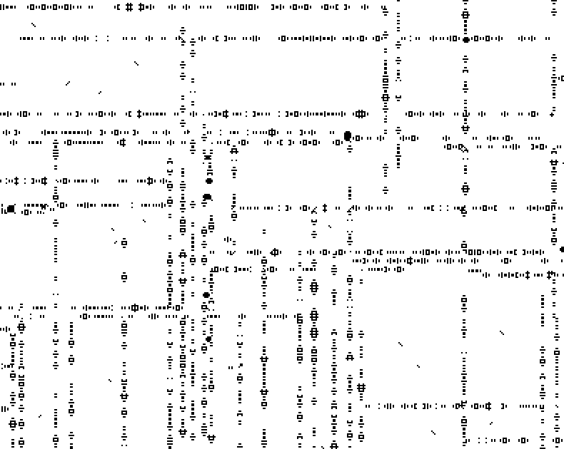
Although I didn’t notice it at the time, this looks very similar to the rectangular Gilbert tessellation! I think that’s not a coincidence. With a fill density of \(\varepsilon\), the most common constellation (connected group of live cells) of the initial configuration will be a single live cell, with density (number of constellations per unit area) approximately \(1/\varepsilon\) . But the isolated cells all die off immediately. The second most common constellations, with density \(\Theta(1/\varepsilon^2)\), have two live cells. If the two cells are diagonally adjacent, they form a small oscillator, and if they are orthogonally adjacent, they form a replicator. The replicators will then grow either horizontally or vertically in both directions until they run into something, usually (but not always) another replicator. When two replicators collide, they tend to form a stable blob that blocks both of them. The one that was there first will usually (but not always) have copies of itself on both sides of the blob, so its line of copies stays more or less unchanged in place. The replicator that arrives second will usually (but not always) be blocked by the first replicator, and stay on one side of the collision point. And when replicators are bounded on both sides by stable blobs, they usually (but not always) turn into stable oscillators, continuing to fill the line they have already marked out. If all of the usual things always happened, we would get a Gilbert tessellation; instead, we get something that looks a lot like a Gilbert tessellation but with typically a constant number of oscillators in its rectangles and with occasional other differences from the expected behavior.
Could this happen for sparse initial conditions of Conway’s Game of Life? Maybe!
In a sequence of papers from 1998 to his 2010 “Emergent Complexity in Conway’s Game of Life”, Nick Gotts has explored the behavior of random Life initial conditions, in the limit as the fill density \(\varepsilon\) goes to zero. We don’t know what happens to these patterns in the long term, but we can say something rigorous about their behavior in the short and medium terms. Here, by “short term” I mean what happens after a constant number of steps, and by “medium term” I mean a number of steps that’s polynomial in \(1/\varepsilon\) with a small-enough exponent.
Initially, near most points of the plane, the nearest objects will be isolated cells, spaced \(\Theta(\varepsilon^{-1/2})\) units from each other (the inverse square root of their density). However, these immediately die off. So in the short term, the nearest objects will usually be “blonks” (blinkers and blocks, generated from initial constellations of three live cells), with density \(\Theta(\varepsilon^3)\) and spacing \(\Theta(\varepsilon^{-3/2})\). More widely scattered are gliders, either generated directly from constellations of five initial live cells, or from R pentominos which create a bounded number of gliders before stabilizing. Both possibilities give the gliders density \(\Theta(\varepsilon^5)\). Even more widely scattered, at density \(\Theta(\varepsilon^{10})\), are the simplest patterns that produce infinite growth rather than stability or simple motion: the block-laying switch engines, generated from initial constellations of ten live cells. These are puffer trains rather than replicators: they have a single live head that lays down a trail of blocks as it moves.
If the field stayed like this throughout the medium term, things would be boring. The gliders and switch engines would typically crash into blonks in \(\Theta(\varepsilon^{-3})\) steps, in most cases stopping their motion. And so one might expect that at numbers of steps with higher exponents, most points would have only stable or low-period debris as their nearest live pattern. Occasionally there would be a trail of a crashed and dead switch engine but these would be very far apart, at a typical distance \(\Theta(\varepsilon^{-5})\), compared to their typical length of \(\Theta(\varepsilon^{-3})\). So from a high-level point of view, these trails would just look like randomly placed line segments rather than forming anything like a motorcycle graph or Gilbert tessellation.
However, what Gotts discovered is that something much more complicated and confusing happens. The gliders (with short-term density \(\varepsilon^5\)) start crashing into blonks, but when they do they sometimes produce one or more new gliders. Those gliders, in turn, might crash into something else and produce even more gliders, perhaps including some that return to the previous crash site. Gotts defines a “standard collision sequence” to be a sequence of events of this type, involving a single initial glider and a widely scattered collection of blonks. There are finitely many different standard collision sequences that involve a given number \(b\) of initial blonks. Any one of these sequences can happen to a given glider with a probability that tends to a constant as the number of time steps goes to \(\Theta(\varepsilon^{-3})\), the expected time for any glider to complete its collision sequence in the absence of interactions with the crash debris of other gliders.
But the crash debris starts to add up, preventing this analysis from actually staying valid all the way to that limiting point. In particular, some standard collision sequences can produce infinite growth patterns like the block-laying switch engine. If we ignored interactions with other gliders and just considered standard collision sequences, it would appear that the density of switch engines constructed in this way would approach \(\varepsilon^5\) as the number of time steps went to \(\varepsilon^{-3}\), and therefore that the density of blocks in switch engine trails would approach \(\varepsilon^2\), much more dense than the density of initial blonks. That can’t happen, and our analysis breaks down. What’s less clear and not rigorously proven is exactly how it breaks down.
One possibility for the breakdown is the following. Switch engines or other puffer engines start being produced in increasing density by standard collision sequences, and they start growing trails of blocks behind them. As their trails grow and the typical distance between the puffers shrinks, at some point these two distances cross over, and the trails become longer than the typical distance. This crossover distance is well below the \(\varepsilon^{-3}\) distance one would expect a puffer to travel before hitting an initial blonk. Once this happens, most puffers will crash into the trail of another puffer, and their trails will divide up space into something resembling a motorcycle graph. (It’s not a Gilbert tessellation, because each puffer starts out moving in a single direction.) The cells of this graph prevent anything else from moving across it, leading to eventual stabilization.
Another possibility is that some other pattern (perhaps initial or perhaps produced by a standard collision sequence) does something quickly enough to disrupt the creation of a motorcycle graph before it happens, or breaks through it after it is constructed. We don’t know what these patterns might look like, but we also don’t know that they don’t exist. Life patterns can do complicated things. Because so much is still unknown, what Gotts actually proves is more cautious: either infinite-growth patterns created from collision sequences eventually cause the total population to be significantly denser than its original density, or the infinite-growth patterns created through standard collision sequences will themselves become more dense than they were in the initial field.
(\(\mathbb{M}\), G+)