Pseudocircles and minimization diagrams
If you've seen Sariel Har-Peled and Timothy Chan's new paper on finding independent sets of pseudodisks, you may be wondering how one might find sets of the non-bounded-aspect-ratio pseudodisks to which their algorithms apply. Or you may be wondering just what is a pseudodisk, anyway. If you're in the former group, you might find one of my own new papers, on minimization diagrams of convex functions (with Kevin Wortman and Matt Dickerson), enlightening. If you're in the latter group, maybe this posting will help.
A disk is just the inside of a circle. Circles have lots of interesting and useful properties but the relevant one here is that any two circles meet in at most two points. This property implies that circles behave nicely in other ways, as well. For instance, the boundary of an intersection of \( n \) disks has at most \( 2n-2 \) arcs (as may be proved using Davenport–Schinzel theory): the four circles below have an intersection bounded by six arcs. In contrast, the best complexity bound we know on the complexity of intersections of the next simplest smooth convex curves, ellipses, is \( O\bigl(n 2^{\alpha(n)}\bigr) \) — see, e.g., my paper with Kevin on dilation, where we used this ellipse bound in the analysis of one of the algorithms.

But circles are not the only families of curves with the two-point-intersection property. For instance, it's also true of any family of shapes formed by scaling and translating (but not rotating) a single strictly-convex curve. In general, a family of simple closed curves in the plane with the same property, that any two curves in the family meet in at most two crossing points, is known as a family of pseudocircles and the insides of these curves are known as pseudodisks.
In our paper on minimization diagrams, the families of curves we looked at come from the following construction: let \( g(x) \) and \( h(y) \) be convex functions, and consider the sets \[ S(a,b;r) = \{(x,y) \mid g(x-a)+h(y-b)=r\}. \] You can think of this as something like a circle, centered at \( (a,b) \), with something like a radius equal to \( r \). For instance, if \( g(x)=x^2 \) and \( h(y)=y^2 \), these shapes really are circles centered at \( (a,b) \), with squared radius \( r \). If \( g \) and \( h \) grow very quickly, as in the example below where both are exponential in the squares of their arguments, you might get curves that are not pseudocircles. But if \( g \) and \( h \) don't grow too quickly (expressed in terms of an ugly inequality of triple derivatives \( g'''g' \lt (g'')^2 \) and \( h'''h' \lt (h'')^2 \)) the resulting shapes are guaranteed to be pseudocircles.

What does this all have to do with the title of our paper, you may be wondering. The pseudocircles are just a means to an end. What we actually care about are minimization diagrams of the functions \( g(x-a)+h(y-b) \): that is, we form a collection of functions of this type, for different centers \( (a,b) \), and we partition the plane into regions within which one of these functions is smaller than all the others. Again, letting \( g(x)=x^2 \) and \( h(y)=y^2 \) as an example, this construction just gives us the Voronoi diagram of the centers. The boundary between two regions in this diagram is known as a bisector; using the pseudocircle property we can show that the bisectors between one region and all the others form pseudolines, curves topologically equivalent to lines that cross each other at most once. And using this pseudoline property we can show that these minimization diagrams behave much like standard Voronoi diagrams: each region is a connected subset of the plane, there are \( O(n) \) boundaries between regions, and the whole thing can be constructed in \( O(n\log n) \) time.
The rest of the title involves a specific choice of convex function to minimize. Or rather, a specific distance function that we want to compute Voronoi diagrams for. We fix a center point \( o \) and (following Ken Clarkson, who gave at UCI this quarter that included this) define the “smoothed distance” \[ d_o(p,q)=\frac{d(p,q)}{d(p,o)+d(o,q)+d(p,q)}, \] the Euclidean distance from \( p \) to \( q \) scaled by the perimeter of triangle \( opq \). If some point \( q \) belongs to the Voronoi region of a site \( p \) for this distance, then the dilation \[ \frac{d(p,o)+d(o,q)}{d(p,q)} \] measuring how far out of your way you would have to go to get from \( p \) to \( q \) via \( o \) is bigger than the dilation from \( q \) to any of the other sites. And although this distance function isn't in the form \( g(x)+h(y) \) needed for our more general results, and isn't even convex, it can be transformed into that form. This transformation was the original reason we started looking at functions of the form \( g(x)+h(y) \).
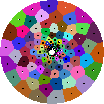
I promised in my report on ACM GIS to say something about Renaissance man Matt Dickerson, one of my co-authors. Not only is Matt a good computational geometry researcher and by all accounts an excellent educator, he's also a renowned Tolkien scholar and literary critic of modern fantasy more generally, a well-traveled and professionally published fly fisherman, a maple syrup farmer, a musician, and a novelist. On top of all of which, he's also a gifted programmer. In response to all this theory, he very quickly threw together a program to compute smoothed distance Voronoi diagrams, to use a \( K \)-means-like algorithm to find highly uniformly spaced points for this distance, and to produce pretty pictures of the results such as the one below. (I was tempted to ask him to throw in my algorithms for choosing contrasting colors but refrained; the colors below are random.)
So, Voronoi diagrams of smoothed distance for (not too widely spaced) point sets behave nicely (the close spacing condition corresponds to the slow growth condition on \( g \) and \( h \)), minimization diagrams of convex functions of the form we consider behave nicely, and their bisectors form an interesting new class of pseudoline arrangements. And it's all because of the pseudocircles.